Hi everyone!
I’m excited to share my new NetLogo project: logolink.
logolink is an R package that simplifies setting up and running NetLogo simulations from R . It provides a modern, intuitive interface that follows tidyverse principles and integrates seamlessly with the tidyverse ecosystem.
The package is available on CRAN and GitHub.

How it Works?
logolink usage is very straightforward. The main functions are:
-
create_experiment: Create NetLogo BehaviorSpace experiment -
run_experiment: Run NetLogo BehaviorSpace experiment
You can install the released version of logolink from CRAN with:
install.packages("logolink")
Along with the package, you will also need NetLogo 7.0.1 or higher installed on your computer. You can download it from the NetLogo website.
The package is feature-complete for BehaviorSpace functionality. The create_experiment() function supports even subexperiments, and run_experiment() supports all four BehaviorSpace output formats: Table, Spreadsheet, Lists, and Statistics.
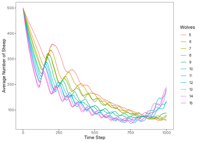
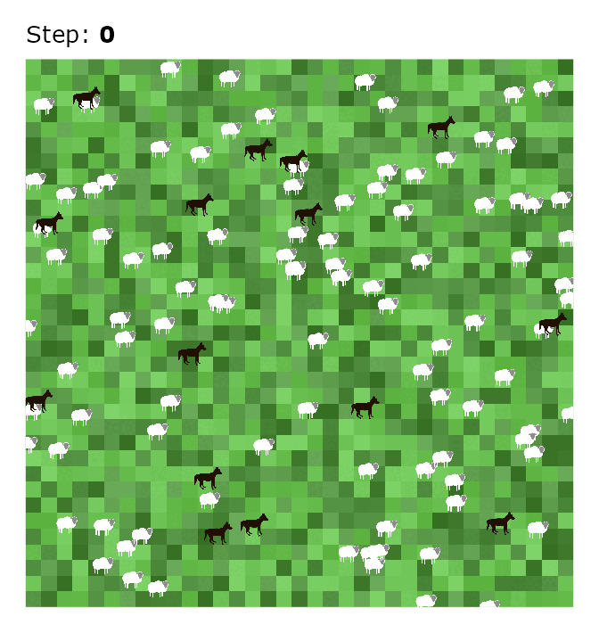
With logolink you can easily perform simulation analyses and capture screenshots of the NetLogo world during simulation runs, all without ever leaving R.
results |> glimpse()
#> List of 2
#>  $ metadata:List of 6
#>   ..$ timestamp       : POSIXct[1:1], format: "2026-01-08 05:11:42"
#>   ..$ netlogo_version : chr "7.0.3"
#>   ..$ output_version  : chr "2.0"
#>   ..$ model_file      : chr "Wolf Sheep Simple 5.nlogox"
#>   ..$ experiment_name : chr "Wolf Sheep Simple Model Analysis"
#>   ..$ world_dimensions: Named int [1:4] -17 17 -17 17
#>   .. ..- attr(*, "names")= chr [1:4] "min-pxcor" "max-pxcor" "min-pycor" "max-pycor"
#>  $ table   : tibble [110,110 × 10] (S3: tbl_df/tbl/data.frame)
#>   ..$ run_number            : num [1:110110] 1 1 1 1 1 1 1 1 1 1 ...
#>   ..$ number_of_sheep       : num [1:110110] 500 500 500 500 500 500 500 500 500 500 ...
#>   ..$ number_of_wolves      : num [1:110110] 5 5 5 5 5 5 5 5 5 5 ...
#>   ..$ movement_cost         : num [1:110110] 0.5 0.5 0.5 0.5 0.5 0.5 0.5 0.5 0.5 0.5 ...
#>   ..$ grass_regrowth_rate   : num [1:110110] 0.3 0.3 0.3 0.3 0.3 0.3 0.3 0.3 0.3 0.3 ...
#>   ..$ energy_gain_from_grass: num [1:110110] 2 2 2 2 2 2 2 2 2 2 ...
#>   ..$ energy_gain_from_sheep: num [1:110110] 5 5 5 5 5 5 5 5 5 5 ...
#>   ..$ step                  : num [1:110110] 0 1 2 3 4 5 6 7 8 9 ...
#>   ..$ count_wolves          : num [1:110110] 5 5 5 5 5 5 5 5 5 5 ...
#>   ..$ count_sheep           : num [1:110110] 500 499 499 498 495 494 492 489 488 486 ...
Learn more at: An Interface for Running NetLogo Simulations • logolink
GitHub Stars are always appreciated! ![]()
Cheers,
Daniel Vartanian